반응형

대칭으로 셀 값 연결은 어떻게 할까?


아래 그림과 같이 12행을 기준으로 대칭으로 값을 연결하고 싶습니다.

C12셀에서 C22셀은 아래쪽으로 그냥 드래그하면 쉽게 연결할 수 있다.

문제는 C2셀에서 C11셀이다.

C2셀에서 C11셀은 거꾸로 연결해야 하는데 좀 쉽게 하는 방법이 있을 까요?


네이버 지식인에 질문을 올렸더니

똭하니 답변이

https://kin.naver.com/qna/detail.nhn?d1id=1&dirId=102020101&docId=403808423&scrollTo=answer1 


대칭으로 셀 값 연결하는 방법?

아래 그림과 같이 12행을 기준으로 대칭으로 값을 연결하고 싶습니다.C12셀에서 아래쪽을 그냥 드래그하면 되는데C2셀에서 C11셀은 거꾸로 연결해야 하는데좀 쉽게 하는 방법이 있을...

kin.naver.com


=INDIRECT("F" & (ROW($B$13)+ROW($B$11)- ROW()))


대칭으로 셀 연결하는 방법.xlsx
0.01MB


2021.09.15 - [엑셀] - 셀번호를 찾아서 적기

반응형
반응형

XLStylesTool

XLStylesTool

"Must have" app for Microsoft Excel users. XLStyles Tool is an Open XML based application, which can analyze and clean out corrupted cell styles in your Excel workbook. XLStyles Tool will also perform analysis of named ranges and report potential issues. User of the tool is able to take actions to remove identified corrupted file content. Files processed by the XLStyles Tool in most cases will show noticeable improvement in file size, opening times, restored ability to support cell format edits (including copy/paste operations) and better overall performance.


Excel 복구 앱 : https://www.microsoft.com/ko-kr/store/apps/xlstylestool/9wzdncrfjptg


XLStylesTool 구매 - Microsoft Store ko-KR

Microsoft Store에서 이 Windows 10, Windows 8.1용 앱을 다운로드하세요. 스크린샷을 보고, 최신 고객 리뷰를 읽고, XLStylesTool에 대한 평점을 비교하세요.

www.microsoft.com


반응형
반응형

파일을 저장하고 다시 열었더니 아래와 같은 경고창이 뜬다.


읽을 수 없는 내용을 복구하거나 제거하여 파일을 열 수 있습니다.


xml파일을 열어보니


<?xml version="1.0" encoding="UTF-8" standalone="yes"?>
<recoveryLog xmlns="http://schemas.openxmlformats.org/spreadsheetml/2006/main"><logFileName>error125160_01.xml</logFileName><summary>'C:\Project\2021\源€?ы븳媛뺣줈?뚯쓬?€媛먯떆???먮┰?앹샊踰?01 援ъ“怨꾩궛??怨꾩궛???묒떇?묒꽦以??먮┰?앹샊踰?援ъ“怨꾩궛??xlsx' ?뚯씪???ㅻ쪟媛€ ?덉뒿?덈떎.</summary><repairedRecords><repairedRecord>蹂듦뎄???덉퐫?? /xl/worksheets/sheet7.xml 遺€遺꾩쓽 蹂닿린</repairedRecord></repairedRecords></recoveryLog>


봐도 무슨 내용인지 모르겠다.


Microsoft Community 사이트에서 아래와 같은 답변을 올려놓았는데 손상이 있는 것으로 예상되니

복구를 해보란다.


Microsoft Community 사이트 를 방문해 주셔서 감사합니다.

문의 하신 Excel 시트 손상에 대해 안내를 드리겠습니다.

말씀해 주신 내용이라면, 이미 문서에 손상이 있는 것으로 예상이 됩니다.

우선 파일 "백업본"을 만든 다음 아래 내용으로 복구를 진행해 보시기 바랍니다.


Excel 손상 복구 : http://answers.microsoft.com/ko-kr/office/forum/office_2010-excel/excel-2003%EC%9E%91%EC%84%B1-%EB%AC%B8%EC%84%9C/b6c188ed-33af-4535-bd33-7f252dea2b20


Excel 복구 앱 : https://labellota.tistory.com/entry/%EC%97%91%EC%85%80%ED%8C%8C%EC%9D%BC-%EB%B3%B5%EA%B5%AC-%EC%95%B1-XLStylesTool


엑셀파일 복구 앱 XLStylesTool

XLStylesTool "Must have" app for Microsoft Excel users. XLStyles Tool is an Open XML based application, which can analyze and clean out corrupted cell styles in your Excel workbook. XLStyles Tool w..

labellota.tistory.com


반응형

'엑셀' 카테고리의 다른 글

대칭으로 셀 값 연결 하는 방법  (0) 2021.10.29
엑셀파일 복구 앱 XLStylesTool  (0) 2021.10.15
엑셀에서 행렬을 3차연립방정식의 풀이  (0) 2021.10.13
유용한 엑셀추가 기능  (0) 2021.10.07
ExcelForFreelancers  (0) 2021.10.06
반응형

엑셀에서 행렬을 3차연립방정식의 풀이


다음과 같은 3차 연립방정식이 있다.

3x + 4y - 2z =3

5x + 4y - z = 5

3x + 3y + z = 5


1. [A][x] = [B]

2. 양변에 [A]의 역행렬을 구한다. MINVERSE

={MINVERSE(D8:F10)}

배열함수이므로 ctrl+shift+enter


3. 양변에 [A]의 역행렬을 곱한다.

[A]-1 * [A]*[x] = [A]-1 * [B]


3. 행렬의 곱 MMULT

[x] = [A]-1 * [B]


x= -1.2359

y=2.411765

z=1.470588


3차연립방정식.xlsx
0.01MB


반응형
반응형

인터넷에서 구해서 유용하게 쓰고 있는 엑셀추가기능들이다.


현재페이지만 인쇄하기

currentpage.xla
0.03MB


이름삭제마법사

esErrNameDelete.xls
0.12MB


remove style

RemoveStyles.xlam
0.02MB


연결셀찾기

유령사냥v10.xla
0.30MB


반응형
반응형

This channel is dedicated to helping Excel Freelancers reach their dreams of financial independence with the ultimate in tricks & tips videos that teach them how to design, create and market Excel based software and sell it forever.

https://youtube.com/c/ExcelForFreelancers


Excel For Freelancers

This channel is dedicated to helping Excel Freelancers reach their dreams of financial independence with the ultimate in tricks & tips videos that teach them how to design, create and market Excel based software and sell it forever.

www.youtube.com


반응형
반응형

순환참조 오류가 있다는 메시지가 나타날때 어떤 곳에서 오류인지 확인하는 방법


수식 > 오류검사 > 순환참조

반응형

'엑셀' 카테고리의 다른 글

유용한 엑셀추가 기능  (0) 2021.10.07
ExcelForFreelancers  (0) 2021.10.06
엑셀 0 값 표시 또는 표시 안 하기  (0) 2021.10.01
Excel에서 그래프 아래의 면적을 계산하는 방법  (0) 2021.09.24
엑셀을 이용한 적분  (0) 2021.09.24
반응형

파일 > 옵션 > 고급 > 0값이 있는 셀에 0표시(Z)


체크하면 0값을 표현하고, 체크를 해지하면 0값을 보이지 않는다.

반응형
반응형

사다리꼴 규칙을 사용하여 그래프 아래 면적 계산


=(C3+C4)/2*(B4-B3)


추세선을 이용하는 방법


가장 일치하는 추세선 선택


y=0.0219x^2+0.7604x+5.1736


F(x)=(0.0219/3)*x^3+(0.7604/2)*x^2+5.1736*x+c


F(1) =(0.0219/3)*1^3+(0.7604/2)*1^2+5.1736*1+c

F(15) = (0.0219/3)*15^3+(0.7604/2)*15^2+5.1736*15+c


면적 = F(15)- F(1)


그래프아래면적계산.xlsx
0.02MB


참고 : https://ko.extendoffice.com/

반응형
반응형

https://myengineeringworld.net/2013/06/integration-trapezoidal-rule.html


Numerical Integration In Excel Using The Trapezoidal Rule - 3 Methods - My Engineering World

Learn how to apply the trapezoidal rule in Excel. Calculate an integral or the area under a curve using 3 different methods (simple formulas, SUMPRODUCT function, and VBA function).

myengineeringworld.net


1st method: Spreadsheet calculations

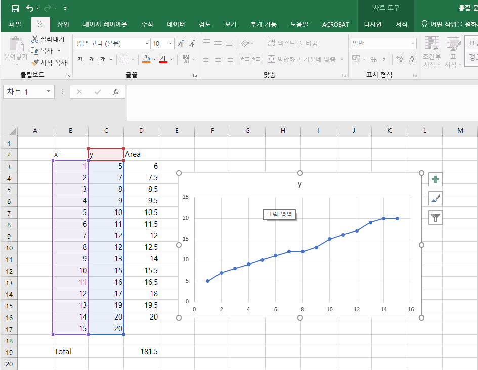
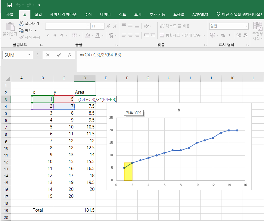
If n points (x, y) from the curve are known, you can apply the previous equation n-1 times and sum the results. For example, in the sample workbook, we had the function y = 4*x^2; we knew 10 points, so we applied the formula 9 times. For the first point the result was (1 – 0)*(4 + 0)/2 = 2, for the second (2 – 1)*(16 + 4)/2 = 10 and so on. The picture above contains the entire set of calculations.


2nd method: SUMPRODUCT formula

With this method, you avoid the intermediate calculations, and by using only one function, you get the result. However, the difficulty level is a little bit higher than the first method (especially if you are new to Excel). The method involves the SUMPRODUCT function, the syntax of which is given below:

SUMPRODUCT(array1, [array2], [array3], …)

The SUMPRODUCT function multiplies the corresponding components in the given arrays and returns the sum of these products. Array1, array2… are the ranges of cells or arrays that you wish to multiply. All arrays must have the same number of rows and columns, and you must enter at least 2 arrays (you can have up to 30 arrays).

The tricky part is the array/range definition. If n curve points (x, y) are known, the function can be written:

In the sample workbook, the SUMPRODUCT function is used with the following ranges:

=SUMPRODUCT(A5:A13-A4:A12;(B5:B13+B4:B12)/2).

In reality, we applied the same function as in method 1, but instead of single cells, we had multiple cells/arrays. The function performs the following calculation:

Without any doubt, the second method is much more straightforward than the first one.


3rd method: Custom VBA function

At your Excel file, switch to VBA editor (ALT + F11), go to the menu Insert Module and add the following code lines.


Option Explicit
Function CurveIntegration(KnownXs As Variant, KnownYs As Variant) As Variant
'---------------------------------------------------------------
'Calculates the area under a curve using the trapezoidal rule.
'KnownXs and KnownYs are the known (x, y) points of the curve.
'Written By:    Christos Samaras
'Date:          12/06/2013
'Last Updated:  21/06/2020
'E-mail:        xristos.samaras@gmail.com
'Site:          https://www.myengineeringworld.net
'---------------------------------------------------------------
'Declaring the necessary variable.
Dim i   As Integer
'Check if the X values belong to a range.
If Not TypeName(KnownXs) = "Range" Then
CurveIntegration = "Xs range is not valid"
Exit Function
End If
'Check if the Y values belong to a range.
If Not TypeName(KnownYs) = "Range" Then
CurveIntegration = "Ys range is not valid"
Exit Function
End If
'Check if the number of X values is equal to the number of Y values.
If KnownXs.Rows.Count <> KnownYs.Rows.Count Then
CurveIntegration = "Number of Xs <> Number of Ys"
Exit Function
End If
'Start with zero.
CurveIntegration = 0
'Loop through all the values.
For i = 1 To KnownXs.Rows.Count - 1
'Check for non-numeric values.
If IsNumeric(KnownXs.Cells(i)) = False Or IsNumeric(KnownXs.Cells(i + 1)) = False _
Or IsNumeric(KnownYs.Cells(i)) = False Or IsNumeric(KnownYs.Cells(i + 1)) = False Then
CurveIntegration = "Non-numeric value in the inputs"
Exit Function
End If
'Apply the trapezoid rule: (y(i+1) + y(i)) * (x(i+1) - x(i)) * 1/2.
'Use the absolute value in case of negative numbers.
CurveIntegration = CurveIntegration + Abs(0.5 * (KnownXs.Cells(i + 1, 1) _
- KnownXs.Cells(i, 1)) * (KnownYs.Cells(i, 1) + KnownYs.Cells(i + 1, 1)))
Next i
End Function


반응형

+ Recent posts